In this post I will talk about:

• The mathematical steps to derive from scratch Principal Component Analysis applied to a basic 2-dimensional example: here
• How to use PCA in real transcriptomic data (RNA-seq) both with Python and R implementation.

What is Principal Component Analysis?

Principal Component Analysis (PCA) is a method designed to decrease the dimensionality of a dataset that contains numerous features. In particular, PCA allow us to summarise the dataset with a smaller number of representative variables which explain most of the information of the original set. PCA serves as a valuable tool for enhancing dataset interpretability and facilitating more straightforward visualization.

Why should we reduce dimentionality?

When dealing with a sizable dataset comprising N data points and M features, creating a single scatterplot becomes impractical. This is due to the inherent limitations of human perception, as we are unable to visualize beyond three dimensions effectively.
What we could do is to create a 2 dimensional scatterplot for each features pairs, for a total of \(\binom{M}{2} = \frac{M(M-1)}{2}\) plots.

This means that for 100 features we will have to inspect at least 5000 scatterplots!!! That’s humanly unfeasible.

Let’s explore a simple example to understand why PCA could help.

Two dimentional example

import numpy as np
import random
import matplotlib.pyplot as plt

random.seed(3)
N=20
x = np.linspace(0,20, num=20)
y = 1+0.5*x + np.random.normal(loc=0.0, scale=2.0, size=N)

mat = np.array([x,y])

fig, ax = plt.subplots(figsize=(3,3),dpi=200)
ax.scatter(x,y, s=5)
plt.xticks(fontsize=4);
plt.yticks(fontsize=4);
ax.set_aspect('equal') # axis are proportional

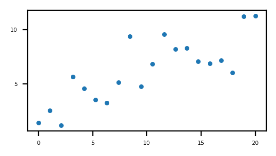Starting points

Scale data

• Values along x are not proportional to values along axis y.
• Values are not centered in 0

We have to make them comparable using a standard scaler (remove the mean of the points and divide by their standard deviation):

The transformed points will have 0 mean and 1 of standard deviation (hence variance since variance is the standard deviation squared)

x_scaled = (x - np.mean(x))/np.std(x)
y_scaled = (y - np.mean(y))/np.std(y)
print(np.std(x_scaled), np.std(y_scaled)) #    1.0 1.0

# Or you can also do it in a vectorized manner:
mat_scaled = (np.transpose(mat) - np.mean(mat, axis=1))/np.std(mat, axis=1)

# Or you can use StandardScaler from sckitlearn
# transpose the original matrix because the scaler wants the observation along the rows and features (x,y) along the columns.
from sklearn.preprocessing import StandardScaler
scaler = StandardScaler()
mat_scaled_sk = scaler.fit_transform(np.transpose(mat)) 

fig, ax = plt.subplots(figsize=(3,3),dpi=200)
ax.scatter(x_scaled, y_scaled, s=5)
plt.xticks(fontsize=4);
plt.yticks(fontsize=4);
ax.set_aspect('equal')
plt.savefig("Figures/PCA_original.pdf", format="pdf", bbox_inches="tight")

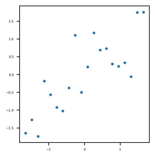Normalized points

Find variance of the projected vectors

The goal is to find a vector that maximise the variance of the projections of the original points. Let’s call \(\textbf{u}\) the unit vector for which we want to project the data onto. We are interested exclusivelly in the direction of this vector, so it’s not important how long it is.

Call \(\textbf{p}_i\) each point observation. In our case we have 20 observations se i goes from 1 to 20.

The projection of \(\textbf{p}_i\) onto \(\textbf{u}\) is:

the second \(\textbf{u}\) is needed because the expression \(\textbf{u}^T \textbf{p}_i\) yelds a scalar value, i.e. the length of the projection of \(\textbf{p}_i\) onto \(\textbf{u}\), so multipling by \(\textbf{u}\) restore the direction of the projection vector.

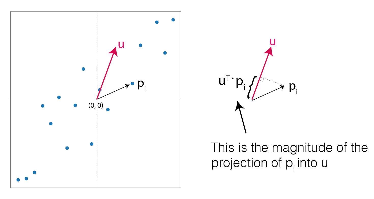Projection of vector p into unit vector u

Iterating this operation for all the observations we have (i=1,…N) we can measure the mean value of these new projected points:

Now we can compute the variance of the projections.
Remember the definition of variance \(\sigma^2\) of a set of points \(\textbf{x}_i\) with \(i \in {1,...,N}\):

Here \(x_i\) is the length (norm) of \(\textbf{x}_i\), therefore when we plug into \(( \textbf{u}^T \textbf{p}_i ) \textbf{u}\) we can drop the last \(\textbf{u}\) since it has length = 1 being a unit vector.

Collect \(\textbf{u}\) outside the brackets:

Expand the square as exploiting this property: \((\textbf{a}^T \textbf{b})^2 = (\textbf{a}^T \textbf{b})(\textbf{b}^T\textbf{a})\)

I can take out of the sum, \(\textbf{u}\) can be taken outside and what remains is the definition of covariance matrix \(S\):

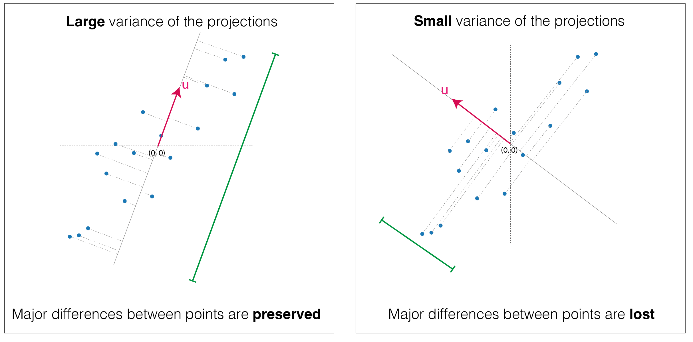Visual representation of large variance and small variance of the projections of the same points

Maximise the variance

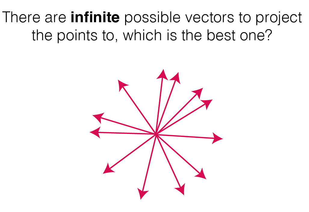
The best vector is the one that yields the maximum variance of the projected point, keeping the most of the variability (i.e. the information) of the original points.

We have to maximise:

considering the costrain

This can be solved using Lagrange multipliers:

This expression is the definition of eigenvectors: \(\textbf{u}\) is an eigenvector of the covariance matrix \(S\) and \(\lambda\) is the eigenvalue.

covariance_matrix = np.cov(mat_scaled, rowvar=False)

# Get Eigen Vectors and Eigen Values
eigen_values, eigen_vectors = np.linalg.eig(covariance_matrix)

# Number of components
num_components=2

# Get highest eigenvalue
sorted_key = np.argsort(eigen_values)[::-1][:num_components]

# Get num_components of Eigen Values and Eigen Vectors
eigen_values, eigen_vectors = eigen_values[sorted_key], eigen_vectors[:, sorted_key]

# Dot product of original data and eigen_vectors are the principal component values
# This is the "projection" step of the original points on to the Principal Component
principal_components=np.dot(mat_scaled, eigen_vectors)

plt.figure(figsize=(8,6))
plt.scatter(principal_components[:,0],principal_components[:,1])
plt.xlabel('First principal component')
plt.ylabel('Second Principal Component')

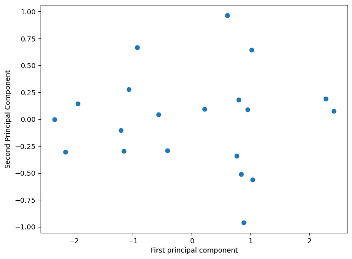PCA transformation of the initial points

In this particular example, there was no need of PCA since we only have two dimensions and the maximum dimensionality reduction achievable is down to just a single dimension. This example was purely didactic, intended to guide through the mathematical procedures.

Now let’s jump into a real case example.

Example on gene expression data

What makes blood cells different from skin cells?
From the genomic point of view, one of the greatest differences is that the activated genes are can be different between the two. Specifically, the intensity of gene activity, known as gene expression, can differ significantly. Some genes may be highly expressed in one tissue but not in another, leading to tissue-specific functions.

The idea in this example is to visualize these differences in gene expression exploiting PCA. I expect that cell lines derived from the same tissue types will be close to each other in the 2 dimensional PCA and at the same time distant from other tissues.

Data download

Gene expression data are downloaded from DepMap database. In the dropdown list you have to select “20Q1” and download CCLE_expression.csv and sample_info.csv. The first file is a matrix where each column is a gene, each row is a cell line (sample) and the values correspond to gene expression values. In particular gene expression is measured with Transcripts Per Million.

Python implementation with scikit-learn

# Import
import pandas as pd
from sklearn.preprocessing import StandardScaler
from sklearn.decomposition import PCA
import seaborn as sns

# rows are samples and genes are columns
df_original = pd.read_csv('CCLE_expression.csv', index_col=0)

# select cell lines for which I have the annotation
annotation = pd.read_csv('sample_info.csv')
to_keep = set(annotation['DepMap_ID']).intersection(set(df_original.index))
annotation_original = annotation.loc[annotation['DepMap_ID'].isin(to_keep),:]

# Take top 5 most frequent classes of lineage for simplicity. 
# There are multiple cell lines from the same lineage
types = annotation_original['lineage_subtype'].value_counts().head(3).index

to_keep = np.unique(annotation_original[annotation_original['lineage_subtype'].isin(types)]['DepMap_ID'])

df = df_original.loc[to_keep, :]
annotation = annotation_original.loc[annotation_original['DepMap_ID'].isin(to_keep),:]
annotation = annotation.reset_index()

# Scale data
scaler = StandardScaler()
scaled_X = scaler.fit_transform(df)

# Performe PCA
pca = PCA(n_components=3)
principal_components = pca.fit_transform(scaled_X)

principal_components = pd.DataFrame(principal_components)
principal_components.index = df.index
principal_components.columns = ['First','Second', 'Third']

# Annotate each sample with the lineage subtype:
# I want to annotate the points with the lineage subtype taken from annotation
# For each element of a this function finds the index of b where the same element is found.
# If it does not exist in b, NA is returned
a = df.index
b = annotation['DepMap_ID'].values
idx = [ int(np.where(b ==i)[0]) if i in b else 'NA' for i in a ]

principal_components['lineage'] = annotation.loc[idx,'lineage'].values
principal_components['lineage_subtype'] = annotation.loc[idx,'lineage_subtype'].values

# Plot
plt.figure(figsize=(8,6))
sns.scatterplot(data = principal_components, x='First', y = 'Second', 
                hue = 'lineage_subtype'
                , palette = ['#EDAE49','#00798C','#D1495B'])
plt.xlabel('First principal component \n(' + format(pca.explained_variance_ratio_[0], '.1%') +' explained variance)' )
plt.ylabel('Second Principal Component \n(' + format(pca.explained_variance_ratio_[1], '.1%')+' explained variance)' );

Python visualization

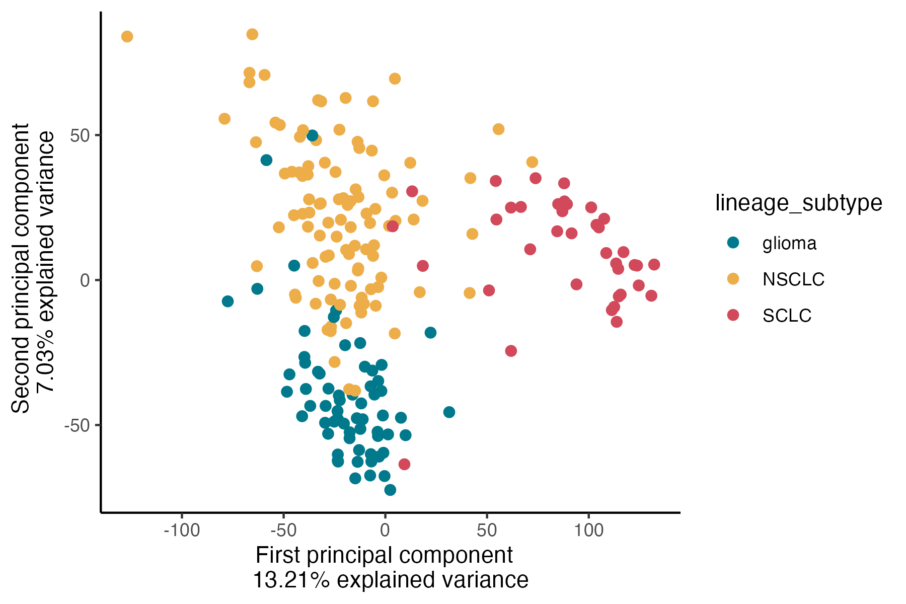
NSCLC = Non-small cell lung cancer (The most frequent lung cancer subtype, 85% of cases)
SCLC = Small-cell lung cancer (The other type of lung cancer type, 15% of cases)
Glioma = Brain tumors

In the figure the red points are cell lines cultured from to SCLC, in yellow from NSCLC and in blue from Glioma.

As you can see there is a “separation” of samples along the first component, highlighting the difference between SCLC and the other two subtypes (13.2% of the total explained variance). On the second component, approximately 7% of the variance is explained. Along the y-axis, when we project points onto it, we observe a clear separation between the two lung subtypes and Glioma.

R implementation with prcomp

library(stats)
library(dplyr)
library(ggplot2)

# Import
df_original = read.csv('~/Downloads/CCLE_expression.csv',  row.names = 1)
annot = read.csv('~/Downloads/sample_info.csv')
annot = subset(annot, lineage_subtype!='')

# Keep only annotated cell lines
annot = subset(annot, DepMap_ID %in% rownames(df_original))
types = sort(table(annot$lineage_subtype), decreasing = T) %>%  head(3)

df = df_original[subset(annot, lineage_subtype%in% names(types))$DepMap_ID,]

# remove genes with zero variance (or standard deviation). 
# Otherwise prcomp raises an error.
sd = apply(df, 2, sd)
df = df[,sd>0]

# Scale e performe PCA at the same time
pca = prcomp(df, scale=T, center=T)
pca_summary = summary(pca)$importance
pca_plot = as.data.frame(pca$x[,c("PC1", "PC2", "PC3")])
pca_plot$lineage_subtype = annot$lineage_subtype[match(rownames(pca_plot), annot$DepMap_ID)]

explained_1 = pca_summary['Proportion of Variance','PC1']
explained_2 = pca_summary['Proportion of Variance','PC2']

# Plot
# I reverse the sign of PC1 and PC2 because it was opposite to python implementation 
# (but principal components are invariant to sign inversion)
ggplot(pca_plot, aes( x = -PC1, y =-PC2, color = lineage_subtype))+
  geom_point(size=2)+
  xlab(paste0('First principal component  \n',round(explained_1*100,2),'% explained variance' ))+
  ylab(paste0('Second principal component  \n',round(explained_2*100,2),'% explained variance' ))+
  scale_color_manual(values = c('NSCLC' ='#EDAE49', 'glioma'= '#00798C', 'SCLC'='#D1495B'))+
  theme_classic()

R visualization

References

• An Introduction to Statistical Learning - James G., Witten D., Trevor H. Tibshirani R.
• ritvikmath videos about PCA help the understanding.